Introduction
Part 2 of the Basin delineation tutorial series focuses on using GRASS7 for creating the initial watershed (or basin) files representing hydrological flow direction and upstream accumulation of each cell in the study region.
Prerequisites
You must have setup GRASS 7 and imported a DEM as described under Installation & Setup in this blog.
Watershed accumulation and basin area
The GRASS raster command r.watershed calculates a variety of hydrological parameters, including the upstream (accumulation) area and the drainage direction of each cell. Note that the accumulation area is calculated as number of cells.
r.watershed can be run assigning a Single Flow Direction (SFD) out of each cell, or Multiple Flow Directions (MFD). MFD is in general preferred and also the default. MFD can be parameterised for determining the flow convergence/divergence, with the recommended default being an average (parameter convergence=5). If you want to avoid negative numbers for upstream area, set the -a flag. r.watershed can be set up to produce a range of hydrologically related layers. For delineating basins you must produce layers for accumulation and drainage.
Single Flow Direction
To apply an SFD flow routing, set the flag -s. In the example below I have set both the -a and -s flags, and I have requested the production of layers for accumulation and drainage. I have set the cutoff threshold at 2000 cells:
With the original DEM (in the mapset PERMANENT):
> r.watershed -as elevation=DEM@PERMANENT accumulation=SFD_upstream drainage=SFD_drainage threshold=2000 –overwrite
With a patched up DEM from part 1:
> r.watershed -as elevation=hydroptfill_DEM accumulation=SFD_upstream drainage=SFD_drainage threshold=2000 –overwrite
It takes a rather long time to run an r.watershed analysis. GRASS thus offers a faster alternative, r.terraflow for massive grids. r.terraflow, however, produces less accurate results and I strongly recommend against using it.
Multiple Flow Directions (MFD)
Omitting the -s flag causes r.watershed to run in default mode, applying an MFD flow routing.
With the original DEM (in the mapset PERMANENT):
> r.watershed -a elevation=DEM@PERMANENT accumulation=MFD_upstream drainage=MFD_drainage threshold=2000 –overwrite
With a patched up DEM from part 1:
> r.watershed -a elevation=hydroptfill_DEM accumulation=MFD_upstream drainage=MFD_drainage threshold=2000 –overwrite
MFD alternative parameterizations
If you want to better capture the full width of wide rivers, you should set a smaller convergence factor for MFD:
> r.watershed -a convergence=1 elevation=DEM@PERMANENT accumulation=MFD01_upstream drainage=MFD01_drainage threshold=2000 –overwrite
Alternatively you can try to beautify flat areas (including wide channels) by setting the -b flag.
> r.watershed -ab convergence=1 elevation=DEM@PERMANENT accumulation=MFDab_upstream drainage=MFDab_drainage threshold=2000 –overwrite
Or even combine a maximum divergence and beautification of flat areas:
> r.watershed -ab convergence=1 elevation=DEM@PERMANENT accumulation=MFDab01_upstream drainage=MFDab01_drainage threshold=2000 –overwrite
Compare upstream accumulation
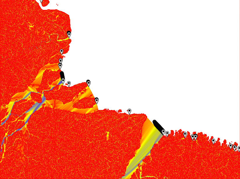
If you look at the accumulation layer, the major Rivers (e.g. the Amazon River) should have the largest accumulation values.
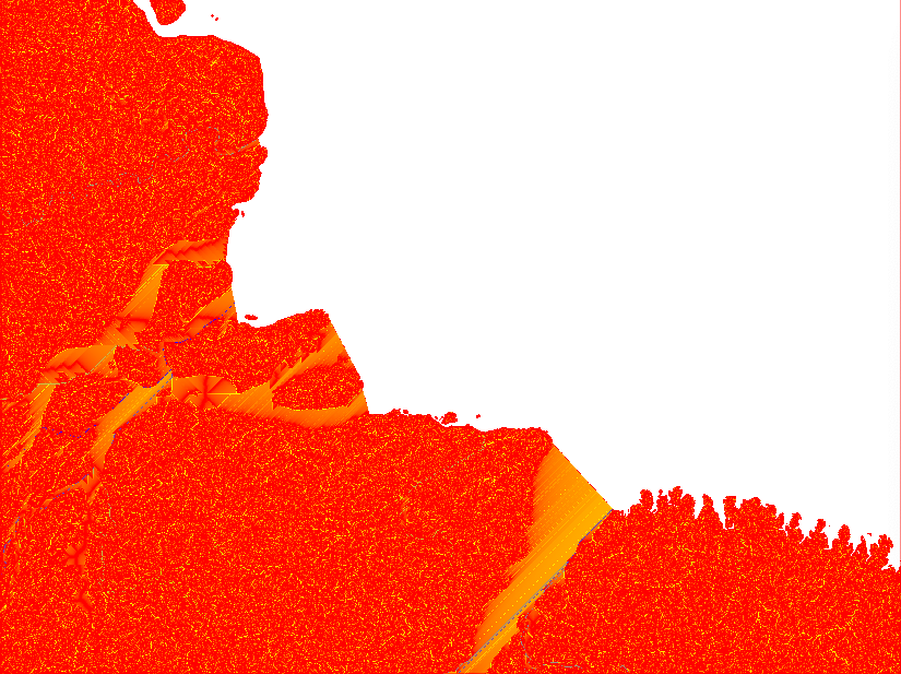

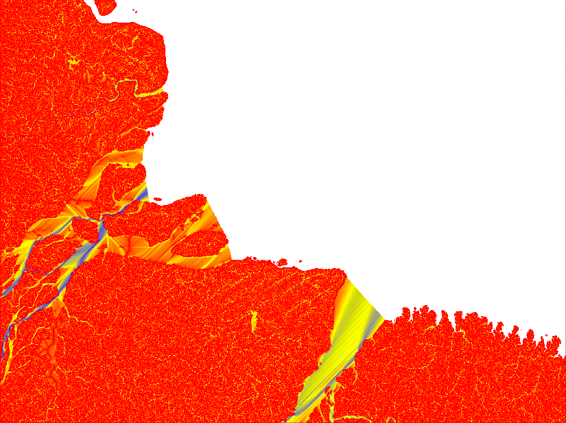
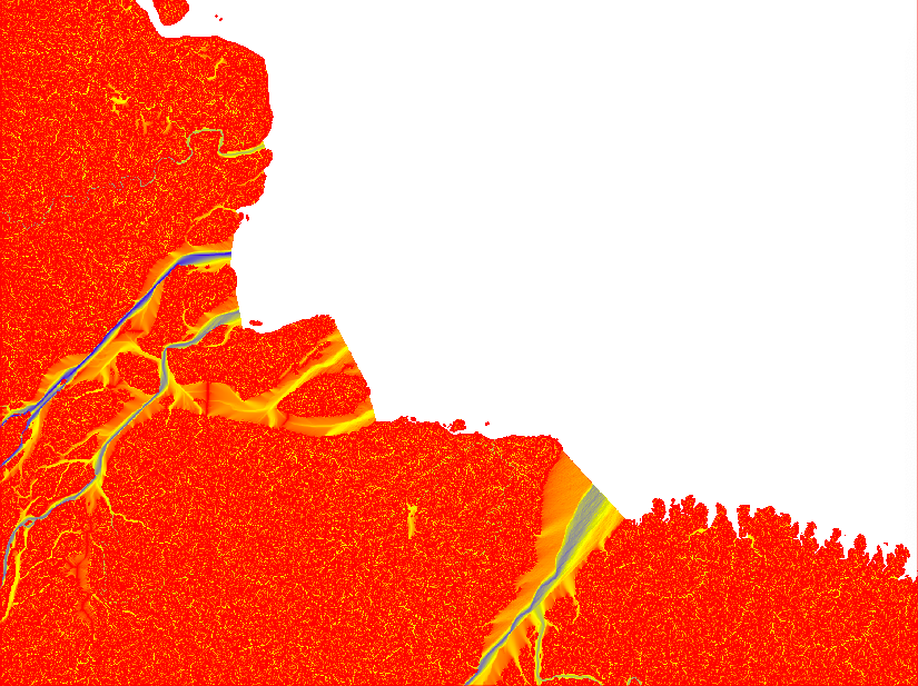
After having compared the result of different Flow Direction parameterisations, I decided to stick with the default settings. In the remaining part of this tutorial series I will rely on default outputs from both SFD and MFD. The reason for using both MFD and SFD is that I want to find all mouths of bifurcating rivers (with MFD) but also all basins that are larger than my set threshhold (regardless of the number of cells though which the basin empties itself in the terminal drainage).
Export upstream layers
You will need the raster layers showing the upstream accumulated areas for inspecting further processing. The upstream layer, however, contains very high numbers and is difficult to visualise. Thus it is better to first get the natural logarithm of the dataset and then export it in byte format. Apply the logarithmic conversion, including a multiplication with 10, with the GRASS command r.mapcalc. Set a colour ramp that is intuitive for interpreting water flow with the command r.colors. I choose red-yellow-blue (ryb). Then export the raster layer with the command r.out.gdal. That is how the 4 maps in the figure above were symbolised.
Start by creating the target directory:
> mkdir -p /Volumes/GRASS2020/GRASSproject/SRTM/region/basin/amazonia/0
Export SFD
The combined commands for exporting a nicely symbolised SFD accumulation layer:
> r.mapcalc "SFD_ln_upstream = 10*log(SFD_upstream)" –overwrite
> r.colors map=SFD_ln_upstream color=ryb
> r.out.gdal -f input=SFD_ln_upstream format=GTiff type=Byte output=/Volumes/GRASS2020/GRASSproject/SRTM/region/basin/amazonia/0/upstream-ln-ryb-SFD_amazonia_0_cgiar-250.tif –overwrite
Export MFD
The combined commands for exporting a nicely symbolised MFD accumulation layer:
> r.mapcalc "MFD_ln_upstream = 10*log(MFD_upstream)" –overwrite
> r.colors map=MFD_ln_upstream color=ryb
> r.out.gdal -f input=MFD_ln_upstream format=GTiff type=Byte output=/Volumes/GRASS2020/GRASSproject/SRTM/region/basin/amazonia/0/upstream-ln-ryb-MFD_amazonia_0_cgiar-250.tif –overwrite
Identify terminal water body
Use r.mapcalc to create a layer where the terminal water body, into which the basins you want to delineate, drain. This is equal to setting all land areas (cells in your DEM layer with valid data) to NULL, and your terminal water body (e.g. the areas assigned with NULL in the DEM) to a value of 1.
With the original DEM (in the mapset PERMANENT):
> r.mapcalc "drain_terminal = if(isnull(‘DEM@PERMANENT’), 1, null())"
With a patched up DEM from part 1:
> r.mapcalc "drain_terminal = if(isnull(‘hydroptfill_DEM’), 1, null())"
Get shoreline
With the terminal water body identified, the shoreline with all the basin outlets will all be found in the neighbouring cells of the water body. In GRASS you can use the proximity analysis tool r.buffer to identify the shoreline from the terminal water body. To capture all shoreline cells set the distance to the length of the side of one cell * sqrt of 2 + plus a little extra. The spatial resolution of the DEM used in this example is 231.6 m. I thus set the distance threshold for the proximity analysis to 330 m.
> r.buffer input=drain_terminal output=shoreline distances=330 units=meters –overwrite
Extract accumulated drainage for shoreline
With both the shoreline and the flow accumulation identified on a per pixel level, you can once again apply r.mapcalc, but this time to mask out the layer with the accumulated upstream area to only include the shoreline (i.e. the potential basin outlets).
> r.mapcalc "shoreline_SFD_flowacc = if((shoreline > 1), SFD_upstream, null())"
> r.mapcalc "shoreline_MFD_flowacc = if((shoreline > 1), MFD_upstream, null())"
Threshold minimum drainage area
The map of the upstream (accumulated) cells masked to show only the shoreline contains the upstream area of every cell along the shoreline, regardless of the upstream area. But you only want the river basins, not the cells that empty directly into the terminal water body or via insignificant water courses. You need to r.reclass the raster layer showing the upstream area of the shoreline to retain only the cells above a given threshold. Remember that the accumulated upstream drainage is given in cells.
r.reclass can be parameterized in different ways, but to keep a memory of the processing it is best to do via a simple text file that is linked in the command. To retain all basins composed to 2000 cells or more, the file looks like this:
2000 thru 99999999 = 1
* = NULL
As the map has a spatial resolution of 231.6 m, 2000 cells equals approximately 100 (107 to be exact) square kilometres. Then run r.reclass with the text file used for parameterisation.
> r.reclass input=shoreline_SFD_flowacc output=basin_SFD_outlets rules=’/Volumes/GRASS2020/GRASSsupport/reclass/reclass_flow_acc_2000.txt’ –overwrite
> r.reclass input=shoreline_MFD_flowacc output=basin_MFD_outlets rules=’/Volumes/GRASS2020/GRASSsupport/reclass/reclass_flow_acc_2000.txt’ –overwrite
Combine the two basin outlet rasters
Distilling the candidate basin outlets to a final set is rather complex - in essence the remaining of parts 2, and parts 3 and 4 are required to get there. To capture all outlets of all basins, the MFD and SFD results need to be joined. Easiest done using r.mapcalc. Alternatively you can patch the vectorised outlets (shown further down) using v.patch.
> r.mapcalc "shoreline_flowacc = if ((shoreline_SFD_flowacc > shoreline_MFD_flowacc), shoreline_SFD_flowacc, shoreline_MFD_flowacc)" –overwrite
> r.reclass input=shoreline_flowacc output=basin_outlets rules=’/Volumes/GRASS2020/GRASSsupport/reclass/reclass_flow_acc_2000.txt’ –overwrite
Vectorize basin outlet candidates
You should now have raster layers with candidate basin outlets. These points are required for the further processing and you need to convert them to vector points. The default suggested processing chain in this tutorial will, however, use the combined SFD and MFD outlets and not the SFD and MFD points. But you can go ahead and convert the latter to vectors anyway. In GRASS you convert raster cells to vector points with the command r.to.vect.
> r.to.vect input=basin_outlets output=basin_outlet_pt type=point –overwrite
> r.to.vect input=basin_SFD_outlets output=basin_SFD_outlet_pt type=point –overwrite
> r.to.vect input=basin_MFD_outlets output=basin_MFD_outlet_pt type=point –overwrite
As mentioned above, you can use v.patch to join the SFD and MFD outlet points. But if you followed the suggested path above you already have a vector layer called basin_outlet_pt.
> v.patch input = basin_SFD_outlet_pt, basin_MFD_outlet_pt output = basin_outlet_pt
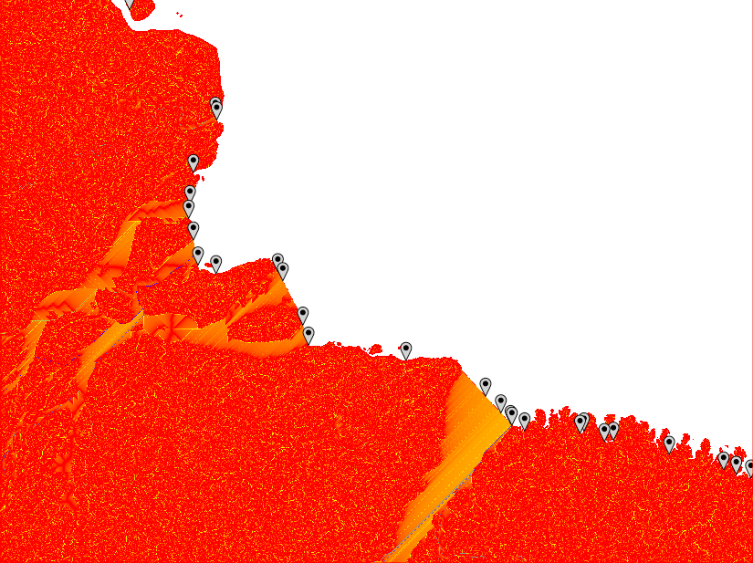
From point outlets to river mouths
From the illustrations above six different problems are evident:
- The MFD analysis identifies multiple adjacent outlet points along wide river mouths of larger basins,
- The MFD analysis only captures basins where the outflow over any single cell is above the threshold, regardless of the size of the basin,
- The SFD analysis does not capture all outlet branches of large rivers that form multiple outlet channels (e.g. in river deltas),
- Separate outlets belonging to the same river (as in 3 above), are not identified as being part of the same basin,
- Both MFD, but in particular SFD, might identify multiple outlet points (or clusters of outlet points regarding MFD) in wide outlet mouths.
- The flow path across flat surfaces differs greatly dependent on the parameterisation of r.watershed.
Problem 1 can be solved by clustering adjacent outlet points, problems 2 and 3 by joining MFD and SFD results. Problem 4 requires analysing the connectivity between adjacent and upstream connected, but along the shoreline topographically separated, river mouths. Problem 5 requires that the complete width of each separate mouth (regardless if part of a delta or not) be identified as a united entity. Issue 6 is only a problem if the identified basins are used for hydrological balancing or modeling (dealt with in parts 3 and 4 of this series).
These problems need to be addressed by combining spatial and database analysis. The solution that I chose accomplishes this by using GRASS and Python scripting. The next section in this part deals with the GRASS spatial analysis for identifying contiguous basin mouths. The Python scripting is the topic of part 3.
Identify contiguous basin mouths
Excluding the sea surface, you could simply reclass the DEM to only retain cells with an elevation of zero for identifying basin mouths. You will then, however, end up with cells along the shoreline that do not constitute a river mouth as well as landlocked regions at sea level. And then there are errors in the DEM and not all basin mouths have an elevation equal 0 (that will be fixed in parts 3 and 4). Instead you need to find all cells at sea level connected to at least one of your candidate outlet points. With the connection either being along the shoreline or via upstream bifurcations. The latter for finding rivers with multiple mouths, like in e.g. river deltas.
Cost growth analysis
Cost growth analysis calculates the accumulated travel cost over a friction surface from predefined starting points. You can use the GRASS cost grow tool r.cost as the first step for finding both the hydrological connectivity between adjacent river mouths and the complete width of the mouths of larger rivers. You have to use all outlet points (from MFD and SFD combined) as starting points and the DEM as a friction surface. Friction at sea surface level (DEM =0) will then be 0, and you let the cost grow analysis travel as long as it is frictionless, i.e. across all of the river mouths.
Identify basin river mouths
If you use the entire DEM for the cost grow analaysis, the result will connect all mouth cells (at sea level), even if not directly connected along the coast. Mouths across a a river delta will be linked (as long as the DEM shows that the water levels equals 0). The r.cost analysis for an entire basin can, however, take a rather long time.
To speed up the processing, you can r.mapcalc the input DEM to only include lower elevations and set higher elevations to NULL. To avoid problems with negative DEM values you can also set these to 0.
With the original DEM (in the mapset PERMANENT):
> r.mapcalc "lowlevel_DEM = if((DEM@PERMANENT <= 0), 0, null())"
With a patched up DEM from part 1:
> r.mapcalc "lowlevel_DEM = if((hydroptfill_DEM <= 0), 0, null())"
If you want to expand the connectivity you can set the “0” of lowlevel_DEM to include also positive elevation (e.g. > r.mapcalc "lowlevel_DEM = if((DEM@PERMANENT <= 2), 0, null())").
Then run r.cost on the more limited DEM. The -n flag retains the null values in the output layer.
> r.cost -n input=lowlevel_DEM output=lowlevel_outlet_costgrow start_points=basin_outlet_pt max_cost=0 –overwrite
To cluster the cells constituting basin mouths use the GRASS command r.clump. Each separate cluster will be assigned a unique id, and you can use that id for identifying river mouths that are separated at the shoreline but joined upstream. Set the -d flag to clump diagonal cells, and then export the raster data source as you will need it to inspect your basins in later parts.
> r.clump -d input=lowlevel_outlet_costgrow output=lowlevel_outlet_clumps –overwrite
> r.out.gdal -f input=lowlevel_outlet_clumps format=GTiff output=/Volumes/GRASS2020/GRASSproject/SRTM/region/basin/amazonia/0/lowlevel-outlet-clumps_amazonia_0_cgiar-250.tif –overwrite
Identify beachfront river mouths
To calculate cost growth for only the shoreline, apply r.mapcalc to extract the DEM only for the shoreline.
With the original DEM (in the mapset PERMANENT):
> r.mapcalc “shoreline_DEM = if((shoreline > 1 && DEM@PERMANENT <= 0), 0, null())” –overwrite
With a patched up DEM from part 1:
> r.mapcalc "shoreline_DEM = if((shoreline > 1 && hydroptfill_DEM <= 0), 0, null())" –overwrite
Then repeat the processing steps for identifying the basin mouths, but for the beachfront mouths.
> r.cost -n input=shoreline_DEM output=shoreline_outlet_costgrow start_points=basin_outlet_pt max_cost=0 –overwrite
> r.clump -d input=shoreline_outlet_costgrow output=shoreline_outlet_clumps –overwrite
> r.out.gdal -f input=shoreline_outlet_clumps format=GTiff output=/Volumes/GRASS2020/GRASSproject/SRTM/region/basin/amazonia/0/shoreline-outlet-clumps_amazonia_0_cgiar-250.tif –overwrite
If you compare the number of clumps reported (at the GRASS commandline), there should be more clumps produced for the shoreline compared to the basin (lowlevel). For the Amazonia region used in the example there are 1065 shoreline clumps and 1037 basin clumps. The difference, 28 mouths, belong to rivers that have two or more separate mouths at the shoreline.
Vectorize beachfront mouths
You should now have clumps of rasters with unique id’s for each separate beachfront mouth. What you ultimately need is a single point in each clump. That is because you want to let all the water from your basin to flow out of that particular cell and none other. To achieve this you need to prepare point data sources in GRASS, and then analyse these in Python.
Vectorize the beachfront mouths with the command r.to.vect.
> r.to.vect input=shoreline_outlet_clumps output=basin_mouth_outlet_pt type=point
Add columns to vector databases
For the database processing in Python, you need to add several columns and fill them with data. You only need to add columns and data to the outlet or mouth vector(s) to use in the next step. The default is to use the basin_mouths_pt point vector. But for convenience the processing of the SFD and MFD point vectors are also included.
Use GRASS vector command v.db.addcolumn to add columns to the vector attribute tables.
> v.db.addcolumn map=basin_mouth_outlet_pt columns=’upstream DOUBLE PRECISION’
> v.db.addcolumn map=basin_mouth_outlet_pt columns=’elevation INT’
> v.db.addcolumn map=basin_mouth_outlet_pt columns=’mouth_id INT’
> v.db.addcolumn map=basin_mouth_outlet_pt columns=’basin_id INT’
or with multiple columns added in one command:
> v.db.addcolumn map=basin_SFD_outlet_pt columns=’upstream DOUBLE PRECISION, elevation INT, mouth_id INT, basin_id INT’
> v.db.addcolumn map=basin_MFD_outlet_pt columns=’upstream DOUBLE PRECISION, elevation INT, mouth_id INT, basin_id INT’
Add basin data to vector databases
To transfer the cell data underlying each point to the vector attribute table, use the GRASS vector command v.what.rast.
> v.what.rast map=basin_mouth_outlet_pt raster=SFD_upstream column=upstream
> v.what.rast map=basin_mouth_outlet_pt raster=DEM@PERMANENT column=elevation
> v.what.rast map=basin_mouth_outlet_pt raster=hydroptfill_DEM column=elevation
> v.what.rast map=basin_mouth_outlet_pt raster=shoreline_outlet_clumps column=mouth_id
> v.what.rast map=basin_mouth_outlet_pt raster=lowlevel_outlet_clumps column=basin_id
> v.what.rast map=basin_SFD_outlet_pt raster=SFD_upstream column=upstream
> v.what.rast map=basin_SFD_outlet_pt raster=DEM@PERMANENT column=elevation
or
> v.what.rast map=basin_SFD_outlet_pt raster=hydroptfill_DEM column=elevation
> v.what.rast map=basin_SFD_outlet_pt raster=shoreline_outlet_clumps column=mouth_id
> v.what.rast map=basin_SFD_outlet_pt raster=lowlevel_outlet_clumps column=basin_id
> v.what.rast map=basin_MFD_outlet_pt raster=MFD_upstream column=upstream
> v.what.rast map=basin_MFD_outlet_pt raster=DEM@PERMANENT column=elevation
or
> v.what.rast map=basin_MFD_outlet_pt raster=hydroptfill_DEM column=elevation
> v.what.rast map=basin_MFD_outlet_pt raster=shoreline_outlet_clumps column=mouth_id
> v.what.rast map=basin_MFD_outlet_pt raster=lowlevel_outlet_clumps column=basin_id
Upload the x and y coordinates to the vector db
Some inherent vector properties can be added to the vector database without prior definition of the column. The command v.to.db creates the column(s) on the fly, for instance for adding point coordinates:
> v.to.db map=basin_mouth_outlet_pt option=coor columns=xcoord,ycoord
> v.to.db map=basin_SFD_outlet_pt option=coor columns=xcoord,ycoord
> v.to.db map=basin_MFD_outlet_pt option=coor columns=xcoord,ycoord
Export basin outlet candidates
Distillation of basin outlets from the candidates is done using a Python script and requires shape files as input. Export the outlet candidates with v.out.ogr.
> v.out.ogr type=point input=basin_mouth_outlet_pt format=ESRI_Shapefile output=/Volumes/GRASS2020/GRASSproject/SRTM/region/basin/amazonia/0/basin-mouth-outlet-pt_drainage_amazonia_0_cgiar-250.shp –overwrite
> v.out.ogr type=point input=basin_SFD_outlet_pt format=ESRI_Shapefile output=/Volumes/GRASS2020/GRASSproject/SRTM/region/basin/amazonia/0/basin-SFD-outlet-pt_drainage_amazonia_0_cgiar-250.shp –overwrite
> v.out.ogr type=point input=basin_MFD_outlet_pt format=ESRI_Shapefile output=/Volumes/GRASS2020/GRASSproject/SRTM/region/basin/amazonia/0/basin-MFD-outlet-pt_drainage_amazonia_0_cgiar-250.shp –overwrite
Virtual direction of basin outflow
The r.watershed analysis is balancing the accumulated input and output through each cell. The results from r.watershed can thus be used for calculating hydrological balances for every cell in a watershed. In wide rivers, including the wide mouths we have dealt with above, the total flow across a section is difficult to retrieve. Also because it depends on the flow direction algorithm. To get the accurate flow along a river, ideally you need a single cell across which all water in the river is forced to pass. To estimate the total outflow of a basin that has a mouth wider than a single cell thus requires a special solution. This section demonstrates how to create a virtual wall across the basin mouth. In the next part a virtual hole will be punched in the wall forcing all flow though a single cell.
Build a virtual wall across the basin mouth
The virtual wall is built by buffering the identified shoreline mouths (shoreline_outlet_clumps) associated with river basins.
Apply an r.buffer analysis the width of 1 diagonal cell (330 m as caclualted above) and starting from the outlet mouths:
> r.buffer input=shoreline_outlet_clumps output=mouth_buffer distances=330 units=meters –overwrite
Overlay the buffer with the map of the terminal drainage, and only retain the buffer cells that fall in the terminal drainage (i.e. on the seaside of the shoreline):
> r.mapcalc "shorewall = if((drain_terminal == 1 && mouth_buffer > 1), 1, null())" –overwrite
Convert the shoreline to vectors - this is the data source you need for the Python processing in the next part.
> r.to.vect input=shorewall output=shorewall_pt type=point
Export the shorewall
Export the point vector version of the shorewall to an ESRI shape file.
> v.out.ogr type=point input=shorewall_pt format=ESRI_Shapefile output=/Volumes/GRASS2020/GRASSproject/SRTM/region/basin/amazonia/0/shorewall-pt_drainage_amazonia_0_cgiar-250.shp –overwrite
Optionally export the shorewall raster map as a geotiff to inspect it in e.g. QGIS.
> r.out.gdal -f format=GTiff type=Byte input=shorewall output=/Volumes/GRASS2020/GRASSproject/SRTM/region/basin/amazonia/0/shorewall_amazonia_0_cgiar-250.tif –overwrite
GRASS shell script
The complete GRASS processing chain in this post (after importing the DEM and creating a new mapset covered in part 1, can be run as a shell script. The shell script omits the trial of different MFD parameterisations discussed above.
# Basin delineation: GRASS watershed analysis

# Watershed accumulation and basin area

r.watershed -as elevation=DEM@PERMANENT accumulation=SFD_upstream drainage=SFD_drainage threshold=2000 --overwrite

# r.watershed -as elevation=hydroptfill_DEM accumulation=SFD_upstream drainage=SFD_drainage threshold=2000 --overwrite

r.watershed -a elevation=DEM@PERMANENT accumulation=MFD_upstream drainage=MFD_drainage threshold=2000 --overwrite

#r.watershed -a elevation=hydroptfill_DEM accumulation=MFD_upstream drainage=MFD_drainage threshold=2000 --overwrite

# Export upstream layers

mkdir -p /Volumes/GRASS2020/GRASSproject/SRTM/region/basin/amazonia/0

r.mapcalc "SFD_ln_upstream = 10*log(SFD_upstream)" --overwrite

r.colors map=SFD_ln_upstream color=ryb

r.out.gdal -f input=SFD_ln_upstream format=GTiff type=Byte output=/Volumes/GRASS2020/GRASSproject/SRTM/region/basin/amazonia/0/upstream-ln-ryb-SFD_amazonia_0_cgiar-250.tif --overwrite

r.mapcalc "MFD_ln_upstream = 10*log(MFD_upstream)" --overwrite

r.colors map=MFD_ln_upstream color=ryb

r.out.gdal -f input=MFD_ln_upstream format=GTiff type=Byte output=/Volumes/GRASS2020/GRASSproject/SRTM/region/basin/amazonia/0/upstream-ln-ryb-MFD_amazonia_0_cgiar-250.tif --overwrite

# Identify terminal water body

r.mapcalc "drain_terminal = if(isnull('DEM@PERMANENT'), 1, null())"

#r.mapcalc "drain_terminal = if(isnull('hydroptfill_DEM'), 1, null())"

# Get shoreline

r.buffer input=drain_terminal output=shoreline distances=330 units=meters --overwrite

# Extract accumulated drainage for shoreline

r.mapcalc "shoreline_SFD_flowacc = if((shoreline > 1), SFD_upstream, null())"

r.mapcalc "shoreline_MFD_flowacc = if((shoreline > 1), MFD_upstream, null())"

# Threshold minimum drainage area

# Create reclass parameterization file
### 2000 thru 99999999 = 1 ###
### * = NULL ###

r.reclass input=shoreline_SFD_flowacc output=basin_SFD_outlets rules='/Volumes/GRASS2020/GRASSsupport/reclass/reclass_flow_acc_2000.txt' --overwrite

r.reclass input=shoreline_MFD_flowacc output=basin_MFD_outlets rules='/Volumes/GRASS2020/GRASSsupport/reclass/reclass_flow_acc_2000.txt' --overwrite

# Combine the two basin outlet rasters

r.mapcalc "shoreline_flowacc = if ((shoreline_SFD_flowacc > shoreline_MFD_flowacc), shoreline_SFD_flowacc, shoreline_MFD_flowacc)" --overwrite

r.reclass input=shoreline_flowacc output=basin_shoreline_outlets rules='/Volumes/GRASS2020/GRASSsupport/reclass/reclass_flow_acc_2000.txt' --overwrite

# Vectorize basin shoreline outlet candidates

r.to.vect input=basin_shoreline_outlets output=basin_outlet_pt type=point --overwrite

r.to.vect input=basin_SFD_outlets output=basin_SFD_outlet_pt type=point  --overwrite

r.to.vect input=basin_MFD_outlets output=basin_MFD_outlet_pt type=point --overwrite

# Identify basin river mouths

### You can change the if conditions to include a wider range of values (e.g. 1 or 2).

r.mapcalc "lowlevel_DEM = if((DEM@PERMANENT <= 0), 0, null())"

#r.mapcalc "lowlevel_DEM = if((hydroptfill_DEM <= 0), 0, null())"

r.cost -n input=lowlevel_DEM output=lowlevel_outlet_costgrow start_points=basin_outlet_pt max_cost=0 --overwrite

r.clump -d input=lowlevel_outlet_costgrow  output=lowlevel_outlet_clumps --overwrite

r.out.gdal -f input=lowlevel_outlet_clumps format=GTiff output=/Volumes/GRASS2020/GRASSproject/SRTM/region/basin/amazonia/0/lowlevel-outlet-clumps_amazonia_0_cgiar-250.tif --overwrite

# Identify beachfront river mouths

r.mapcalc "shoreline_DEM = if((shoreline > 1 && DEM@PERMANENT <= 0), 0, null())" --overwrite

#r.mapcalc "shoreline_DEM = if((shoreline > 1 && hydroptfill_DEM <= 0), 0, null())" --overwrite

r.cost -n input=shoreline_DEM output=shoreline_outlet_costgrow start_points=basin_outlet_pt max_cost=0 --overwrite

r.clump -d input=shoreline_outlet_costgrow output=shoreline_outlet_clumps --overwrite

r.out.gdal -f input=shoreline_outlet_clumps format=GTiff output=/Volumes/GRASS2020/GRASSproject/SRTM/region/basin/amazonia/0/shoreline-outlet-clumps_amazonia_0_cgiar-250.tif --overwrite

### From this point the separate SFD and MFD data sources are not needed for a combined solutions. The coding is however included for convenience. ###

# Vectorize shoreline mouths

r.to.vect input=shoreline_outlet_clumps output=basin_mouth_outlet_pt type=point

# Add columns to vector databases

v.db.addcolumn map=basin_mouth_outlet_pt columns='upstream DOUBLE PRECISION'

v.db.addcolumn map=basin_mouth_outlet_pt columns='elevation INT'

v.db.addcolumn map=basin_mouth_outlet_pt columns='mouth_id INT'

v.db.addcolumn map=basin_mouth_outlet_pt columns='basin_id INT'

# or with multiple columns added in one command

v.db.addcolumn map=basin_SFD_outlet_pt columns='upstream DOUBLE PRECISION, elevation INT, mouth_id INT, basin_id INT'

v.db.addcolumn map=basin_MFD_outlet_pt columns='upstream DOUBLE PRECISION, elevation INT, mouth_id INT, basin_id INT'

# Add basin data to vector databases

v.what.rast map=basin_mouth_outlet_pt raster=SFD_upstream column=upstream

v.what.rast map=basin_mouth_outlet_pt raster=DEM@PERMANENT column=elevation

#v.what.rast map=basin_mouth_outlet_pt raster=hydroptfill_DEM column=elevation

v.what.rast map=basin_mouth_outlet_pt raster=shoreline_outlet_clumps column=mouth_id

v.what.rast map=basin_mouth_outlet_pt raster=lowlevel_outlet_clumps column=basin_id

v.what.rast map=basin_SFD_outlet_pt raster=SFD_upstream column=upstream

v.what.rast map=basin_SFD_outlet_pt raster=DEM@PERMANENT column=elevation

#v.what.rast map=basin_SFD_outlet_pt raster=hydroptfill_DEM column=elevation

v.what.rast map=basin_SFD_outlet_pt raster=shoreline_outlet_clumps column=mouth_id

v.what.rast map=basin_SFD_outlet_pt raster=lowlevel_outlet_clumps column=basin_id

v.what.rast map=basin_MFD_outlet_pt raster=MFD_upstream column=upstream

v.what.rast map=basin_MFD_outlet_pt raster=DEM@PERMANENT column=elevation

#v.what.rast map=basin_MFD_outlet_pt raster=hydroptfill_DEM column=elevation

v.what.rast map=basin_MFD_outlet_pt raster=shoreline_outlet_clumps column=mouth_id

v.what.rast map=basin_MFD_outlet_pt raster=lowlevel_outlet_clumps column=basin_id

# Upload the x and y coordinates to the vector db

v.to.db map=basin_mouth_outlet_pt option=coor columns=xcoord,ycoord

v.to.db map=basin_SFD_outlet_pt option=coor columns=xcoord,ycoord

v.to.db map=basin_MFD_outlet_pt option=coor columns=xcoord,ycoord

# Export basin outlet candidates

v.out.ogr type=point input=basin_mouth_outlet_pt format=ESRI_Shapefile output=/Volumes/GRASS2020/GRASSproject/SRTM/region/basin/amazonia/0/basin-mouth-outlet-pt_drainage_amazonia_0_cgiar-250.shp --overwrite

v.out.ogr type=point input=basin_SFD_outlet_pt format=ESRI_Shapefile output=/Volumes/GRASS2020/GRASSproject/SRTM/region/basin/amazonia/0/basin-SFD-outlet-pt_drainage_amazonia_0_cgiar-250.shp --overwrite

v.out.ogr type=point input=basin_MFD_outlet_pt format=ESRI_Shapefile output=/Volumes/GRASS2020/GRASSproject/SRTM/region/basin/amazonia/0/basin-MFD-outlet-pt_drainage_amazonia_0_cgiar-250.shp --overwrite

# Build a virtual wall across the basin mouths

r.buffer input=shoreline_outlet_clumps output=mouth_buffer distances=330 units=meters --overwrite

r.mapcalc "thickwall = if((drain_terminal == 1 && mouth_buffer > 1), 1, null())" --overwrite

r.out.gdal -f format=GTiff type=Byte input=thickwall output=/Volumes/GRASS2020/GRASSproject/SRTM/region/basin/amazonia/0/thickwall_amazonia_0_cgiar-250.tif --overwrite

# Shrink the thickwall to 1 cell width

r.mapcalc "drain_terminal_remain = if((drain_terminal == 1),  if ((isnull(thickwall)),1, null() ),null() ) " --overwrite

r.out.gdal -f format=GTiff type=Byte input=drain_terminal_remain output=/Volumes/GRASS2020/GRASSproject/SRTM/region/basin/amazonia/0/drain-terminal-remain_amazonia_0_cgiar-250.tif --overwrite

r.buffer input=drain_terminal_remain output=mouthshoreline distances=330 units=meters --overwrite

r.out.gdal -f format=GTiff type=Byte input=mouthshoreline output=/Volumes/GRASS2020/GRASSproject/SRTM/region/basin/amazonia/0/mouthshoreline_amazonia_0_cgiar-250.tif --overwrite

r.mapcalc "shorewall = if((mouthshoreline > 1 && thickwall == 1), 1, null())" --overwrite

r.out.gdal -f format=GTiff type=Byte input=shorewall output=/Volumes/GRASS2020/GRASSproject/SRTM/region/basin/amazonia/0/shorewall_amazonia_0_cgiar-250.tif --overwrite

r.to.vect input=shorewall output=shorewall_pt type=point --overwrite

v.out.ogr type=point input=shorewall_pt format=ESRI_Shapefile output=/Volumes/GRASS2020/GRASSproject/SRTM/region/basin/amazonia/0/shorewall-pt_drainage_amazonia_0_cgiar-250.shp --overwrite

r.out.gdal -f format=GTiff type=Byte input=shorewall output=/Volumes/GRASS2020/GRASSproject/SRTM/region/basin/amazonia/0/shorewall_amazonia_0_cgiar-250.tif --overwrite

# Fill up the original DEM with the holes created from the difference between thickwall and shorewall

r.mapcalc "fillholeDEM = if ((thickwall==1 && isnull(mouthwall)),1, null() ) " --overwrite

r.out.gdal format=GTiff type=Byte input=fillholeDEM output=/Volumes/GRASS2020/GRASSproject/SRTM/region/basin/amazonia/0/fillholeDEM_amazonia_0_cgiar-250.tif --overwrite
Next step
The next step requires in depth analysis of database records and spatial relations. I do not know how to accomplish that using standard GIS commands. The next step thus requires Python scripting.